
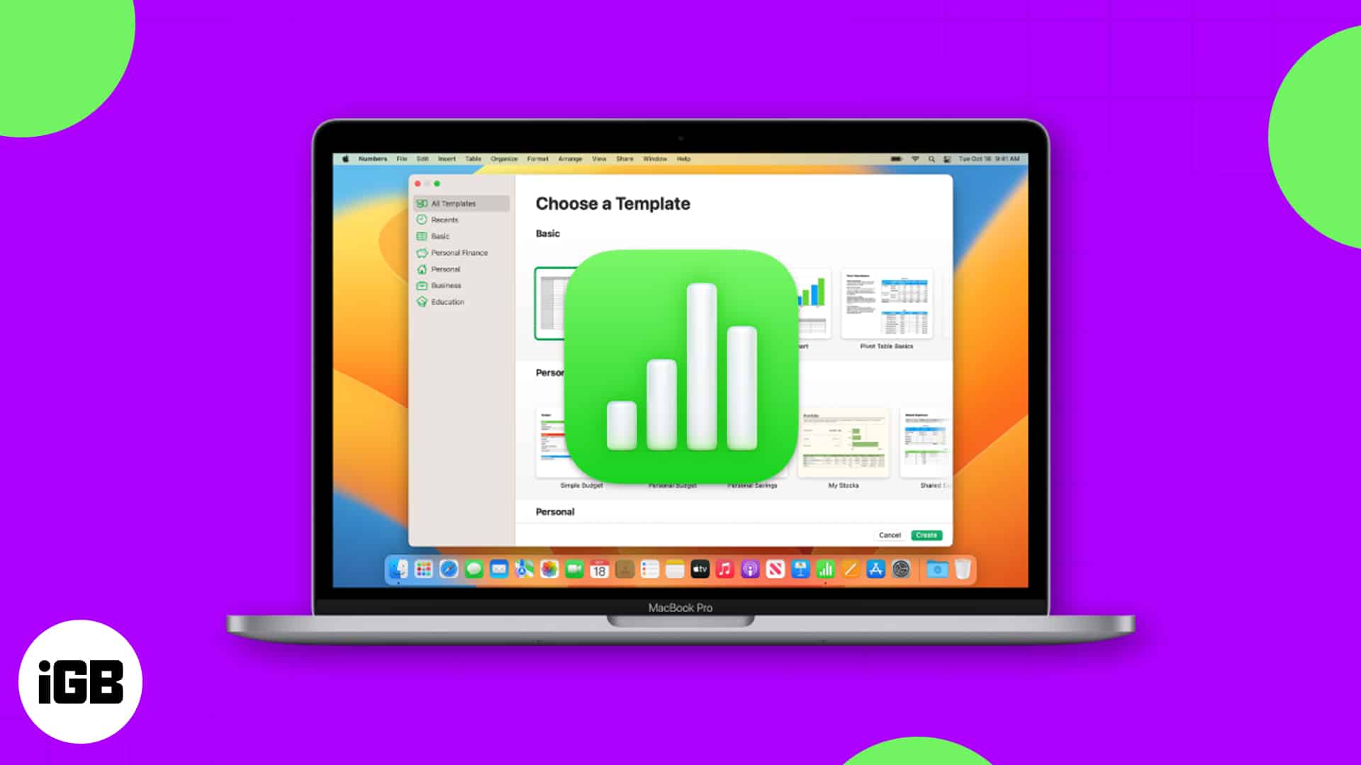
Unsure how you can get began in Apple Numbers on Mac? For enterprise and private use, Numbers is a helpful spreadsheet software that comes with macOS. However there’s extra causes to make use of Numbers – it presents helpful options which may simply make it one among your favourite go-to apps.
We’ll stroll you thru a number of ideas for utilizing Apple Numbers on Mac. From beginning with a template to making use of conditional highlighting, open Numbers and observe alongside!
1. How one can begin with a template in Numbers
If you would like a jumpstart in your Numbers spreadsheet, you can begin with a template. You’ll discover a first rate collection of private, enterprise, and academic templates for frequent duties.
- Launch the Numbers app in your Mac and choose New Doc.
If you have already got the app open, go to File within the menu bar and select New. - Use the navigation on the left aspect of the next display to select a class or select All Templates to overview them. You’ll be able to create every part from a activity guidelines to a family funds to a category schedule.
- If you see the one you need, choose it and click on Create on the backside proper.
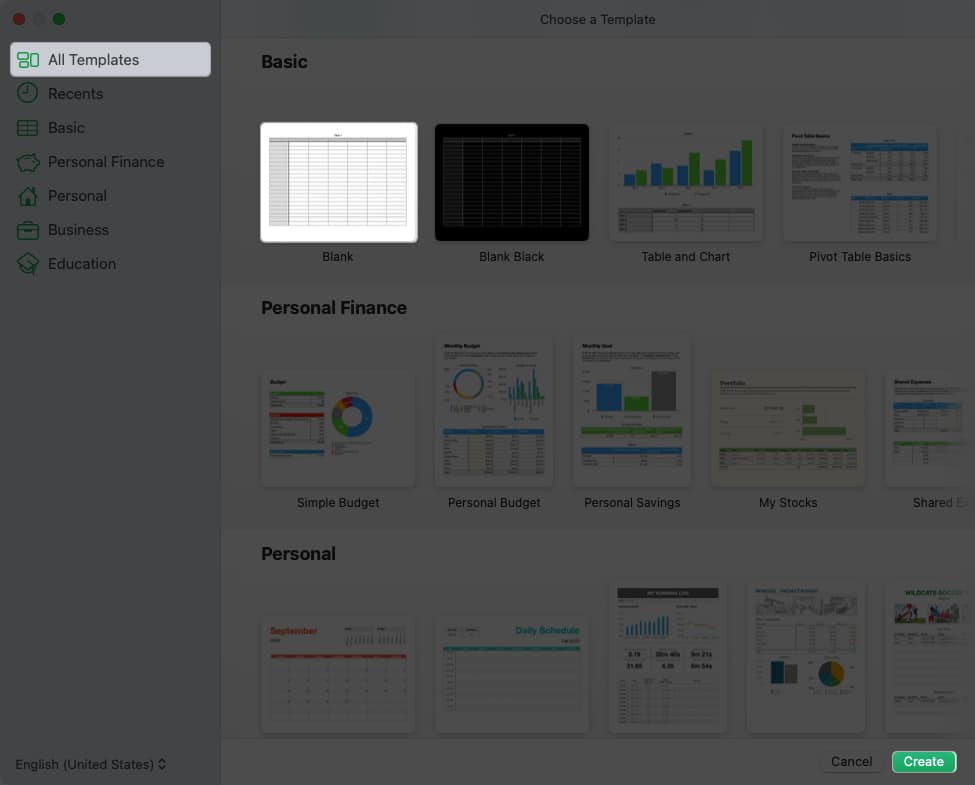
As soon as the template opens, merely add your individual information. You may also make edits to the template formatting to tailor it to your wants.
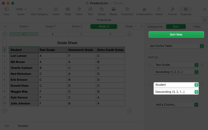
2. How one can type information in Numbers
When you may have a spreadsheet that features plenty of information, manually manipulating it may be time-consuming and also you run the danger of errors. As a substitute, you should utilize the type characteristic for the info in your sheet.
- Choose the sheet you wish to type, click on the Set up button on the high proper nook, and select the Type tab.
- In case you solely wish to type explicit information, choose these rows after which decide Type Chosen Rows within the high drop-down field within the sidebar. In any other case, you’ll be able to select Type Complete Desk.
- Within the Type by part, decide the column you wish to type by within the drop-down field. Beneath, you’ll be able to then select Ascending or Descending order.
- In case you’d prefer to type by one other column, select it together with the order beneath the primary type settings you decide.
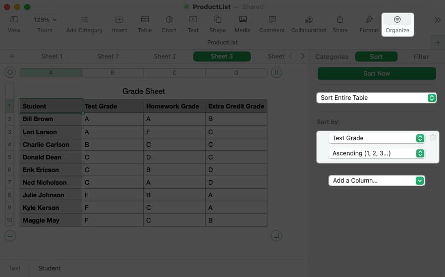
- You must see your information routinely sorted, however in case you proceed so as to add extra columns to type by, click on Type Now on the high of the sidebar.
3. How one can add a hyperlink in Numbers
Possibly you’d like to incorporate a reference to a different sheet or a fast approach to go to an internet site. You’ll be able to add a hyperlink in Numbers to a sheet, electronic mail deal with, internet web page, or telephone quantity. Then, with a easy click on of the hyperlink, you’ll be able to open the sheet, compose an electronic mail, go to the web page, or make a telephone name.
- Choose the content material inside the cell you wish to hyperlink by double-clicking the textual content or dragging your cursor by means of it. In case you solely choose the cell, you’ll discover that the hyperlink choices shall be
- Go to Format within the menu bar, transfer your cursor to Add Hyperlink, and select an choice from the pop-out menu. unavailable.
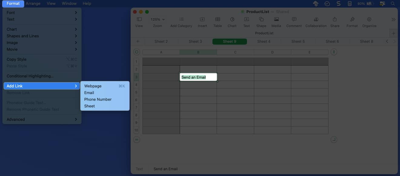
- When the small window seems, add the data for the hyperlink. For instance, enter the URL for an internet web page or quantity for a telephone name. You may also alter the Show textual content if mandatory.
- Use the button on the underside proper per the kind of hyperlink you choose to use the hyperlink to the content material.
To make adjustments to the hyperlink or take away it later, choose Format within the menu bar and decide Edit Hyperlink or Take away Hyperlink.
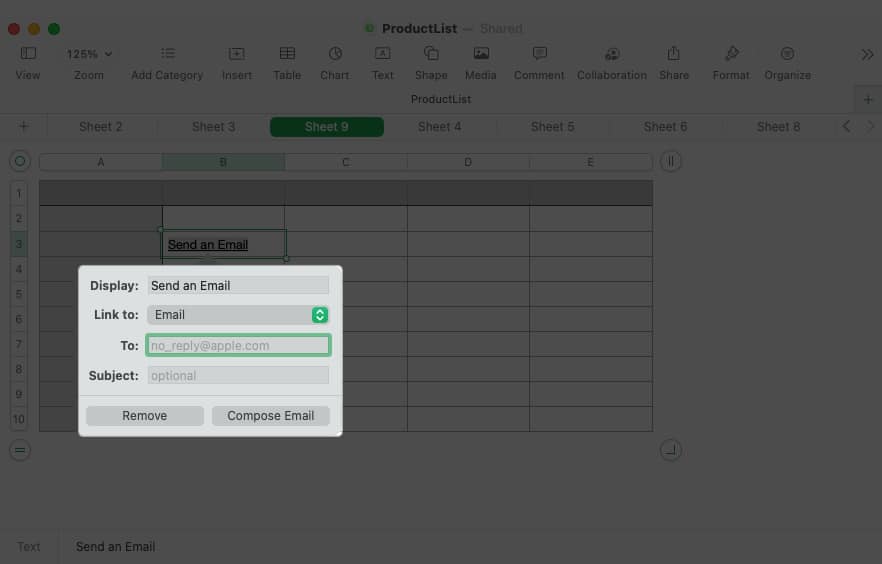
4. How one can create a chart in Numbers
Charts and graphs are terrific visuals for displaying information. They assist you to see highs and lows, traits, or patterns at a look. In Numbers, you’ll be able to select from 2D, 3D, and interactive charts.
- Choose the info you wish to embrace within the chart.
- Both click on the Chart button within the toolbar or Insert within the menu bar and transfer to Chart.
- You’ll see all the chart sorts you’ll be able to decide from together with bar, column, pie, scatter, and extra. Select the kind and also you’ll see the chart pop proper into your sheet.
- If you edit the info in your sheet, your chart routinely updates.
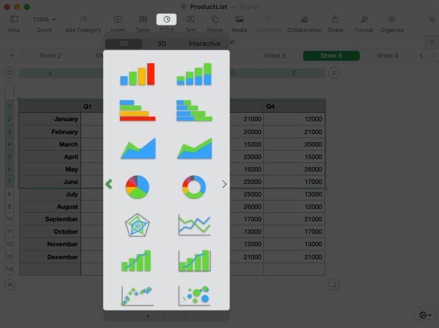
- To customise the looks, choose the chart and click on Format on the highest proper. You’ll be able to then select a special shade scheme, alter the axes, add information labels, and extra.
- To alter the info you wish to embrace, choose the chart and click on Edit Information References on the backside of the chart.
5. How one can carry out easy calculations in Numbers
One of the frequent belongings you’ll doubtless do in your Numbers sheet is to carry out calculations. Fortunately, you’ll be able to add, common, or get the utmost quantity from an information set in simply a few clicks.
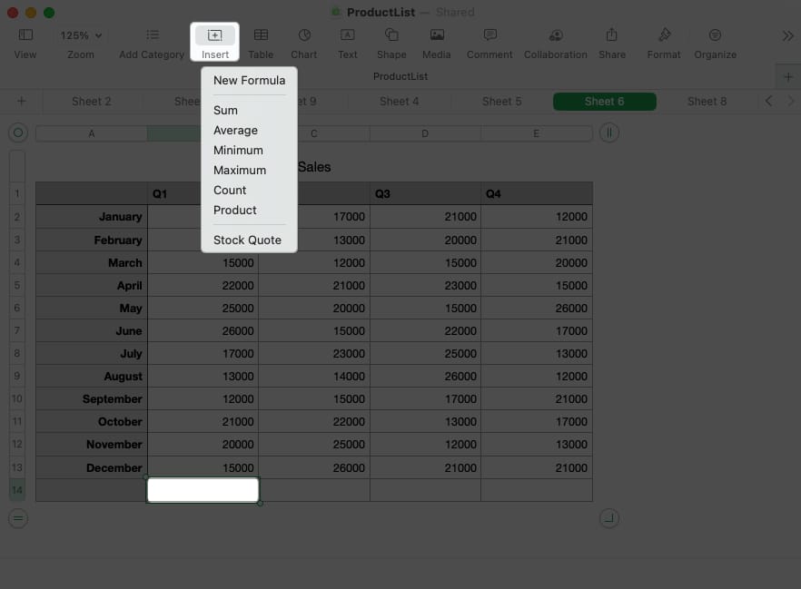
- Go to the cell the place you need the outcomes of the calculation.
- Both choose Insert within the toolbar or use Insert within the menu bar to decide on Method.
- Then, decide the calculation you wish to use.
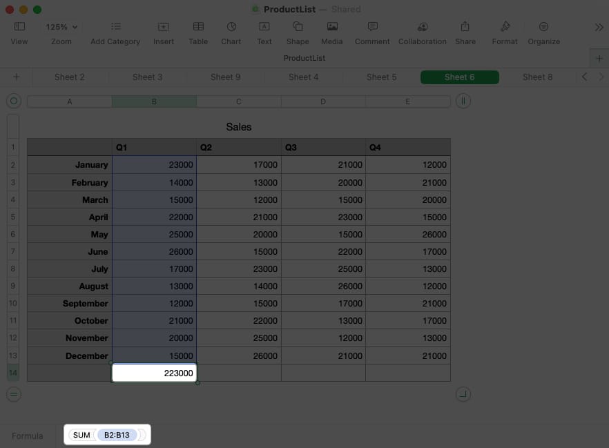
You’ll see Numbers use the values within the column in case you use the underside cell or row in case you use the far-right cell to carry out the calculation for you.
To edit the components for the calculation, double-click the cell to show the components bar. Then, make your adjustments and use the checkmark in inexperienced to reserve it.
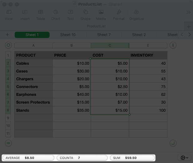
View calculations at a look
Possibly you wish to use one among these calculations, however not essentially add it to your sheet. As a substitute, you’ll be able to show one or all of them on the backside of the window.
- Choose a gaggle of cells containing values in your sheet. Then, click on the gear button that shows within the backside proper nook of the window.
- Select the calculations you wish to show which locations a checkmark subsequent to every one.
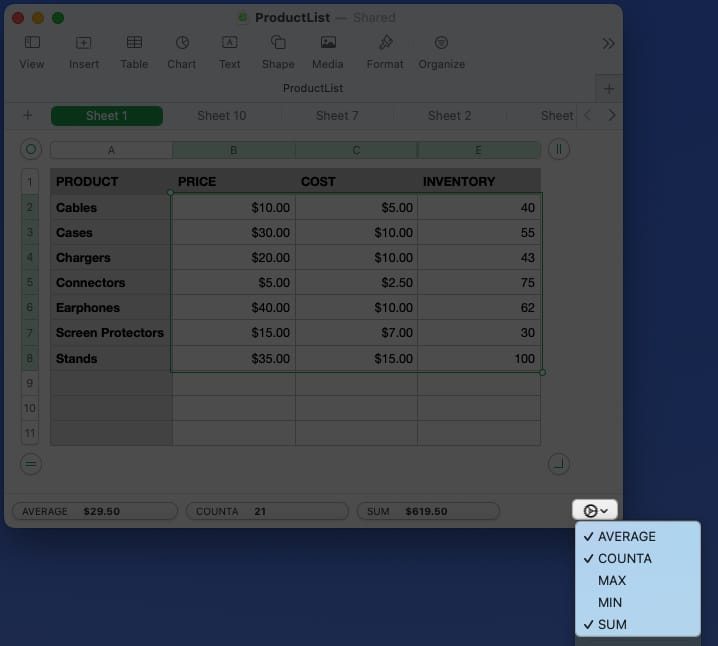
- Then, when you choose a number of cells within the sheet, you’ll see the calculation(s) on the backside with nothing greater than a look.
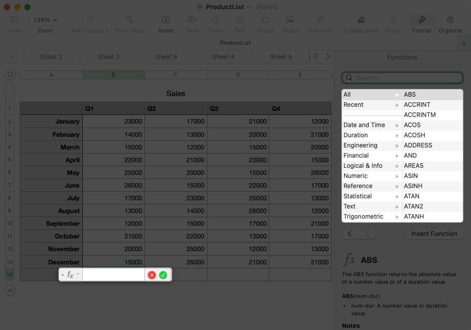
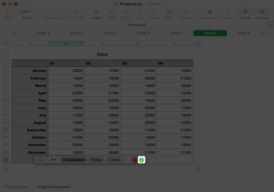
6. How one can insert formulation in Numbers
If you carry out the straightforward calculations described above, these equations use formulation. With Numbers, you’ll be able to transcend the fundamentals by coming into superior formulation and utilizing a wide range of capabilities.
As a result of formulation and capabilities in Numbers may spawn a brilliant prolonged article, we’ll simply cowl the necessities right here.
- To enter a components, sort the equal signal (=) within the cell to show the components bar.
- Sort the components you wish to use into the components bar. In case you begin your components with a perform, you’ll discover strategies on the backside. In case you select one, you’ll obtain prompts contained in the components bar that enable you full the components accurately. Merely exchange the prompts together with your information.
- Moreover, you’ll be able to open the Format sidebar to get extra assist with capabilities. You’ll be able to seek for one, get particulars on its makes use of, and click on Insert Perform to position it in your components.
- If you end coming into the components, press the checkmark in inexperienced to use it and acquire your end result.
Tip: If you would like a fast view of the components, choose the cell, and also you’ll see the components displayed on the backside of the window.
Method and performance examples
Let’s have a look at a few frequent formulation utilizing capabilities in Numbers.
Utilizing the IF perform, you’ll be able to return a end result for a real or false situation. For instance, if the quantity in cell B2 is larger than 20,000, return Sure, in any other case, return No. Right here’s the components you’d use and the way it seems within the bar on the backside:
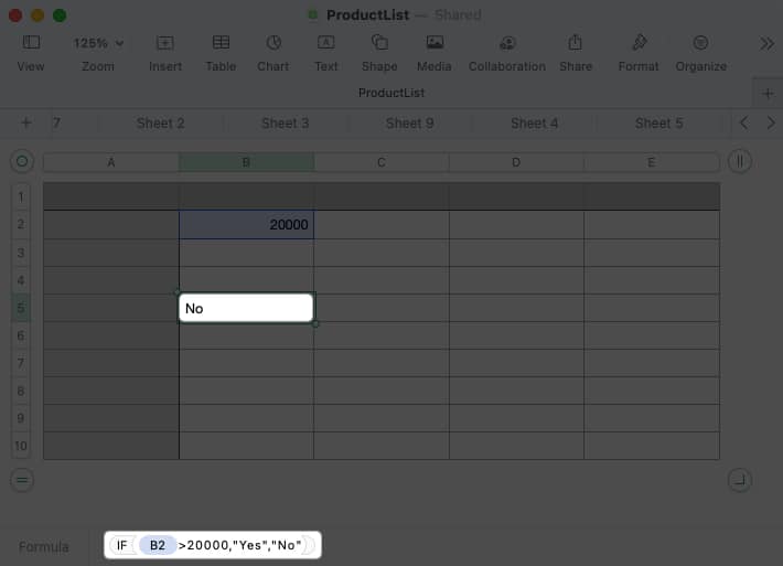
IF(B2>20000,”Sure”,”No”)
Utilizing the CONCAT perform, you’ll be able to mix textual content from completely different cells. As an illustration, you’ll be able to be a part of the primary title in cell B2 and the final title in cell C2 with the lead to cell D2. You may also embrace an area (inside quotes) between the names. Right here’s the components and the way it seems to be within the bar on the backside:

CONCAT(B2,” “,C2)
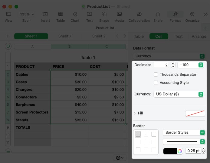
7. How one can apply cell formatting in Numbers
Relying on the kind of information you enter in Numbers, you might have considered trying or must format it as such.
As an illustration, you may want numbers formatted as foreign money, a proportion, or a date. Whereas Numbers presents an Computerized formatting choice, you’ll be able to select and customise explicit information sorts.
- Choose the cell or vary of knowledge and click on Format to open the sidebar.
- Go to the Cell tab and open the Information Format drop-down field to select the info sort.
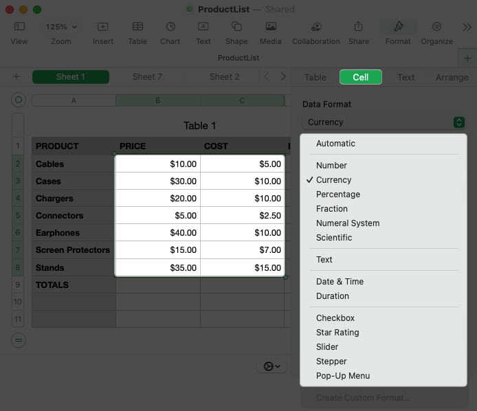
- Optionally, you’ll be able to alter the extra formatting that shows beneath the kind. For instance, in case you select Foreign money, you’ll be able to select the foreign money sort, change the decimal locations, and embrace a thousand separator.
8. How one can use interactive formatting in Numbers
Together with formatting the info, you’ll be able to format a cell with an interactive merchandise like a checkbox or slider. This provides you a fast and simple approach to mark off duties, select values, or add a score.
- Choose the cell or vary and click on Format to open the sidebar.
- Go to the Cell tab and open the Information Format drop-down field to select one among these interactive formatting sorts on the backside of the checklist.
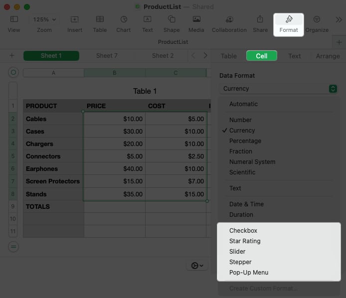
- Checkbox: Click on the field to position a checkmark in it. When checked, the worth is True and when unchecked, the worth is False.
- Star score: Choose a dot to mark that variety of stars for a score system. You’ll be able to select from zero to 5 stars.
- Slider: Use a vertical slider to pick out a worth. After you select Slider within the drop-down field, add the minimal, most, and increments. You may also decide a selected information format resembling quantity, foreign money, or proportion.
- Stepper: A Stepper works like a Slider besides you employ arrows to extend or lower the worth.
- Pop-up menu: Create your individual pop-up menu by including the objects within the sidebar. Then, choose the arrow to the appropriate to open the pop-up menu and decide an merchandise.
9. How one can use autofill in Numbers
Autofill is a incredible characteristic that may be a real time saver. With it, you’ll be able to drag from a number of cells to fill further cells with the identical worth, a sample, or a components.
One of the best ways to clarify how you can use autofill is with a number of examples.
Autofill the identical worth
Right here, we wish to copy the identical worth all the way down to the final three cells within the column. When you choose the cell, hover your cursor over it and also you’ll see a yellow dot show. Drag that dot downward and launch to fill the cells with the identical worth.
Autofill a sample
Subsequent, we wish to checklist the months of the 12 months. Fairly than typing all of them manually, you’ll be able to choose the cell containing “January” and drag the yellow dot all the way down to fill within the remaining months.
Autofill a components
If you enter a components or calculation right into a cell that you just wish to use in one other, you’ll be able to copy and paste the components with autofill. Numbers routinely updates the cell references in order that they apply to the right cells.
Right here, we have now our complete for Q1. We drag the cell with that SUM components to the cells throughout the row to acquire the totals for the remaining quarters.
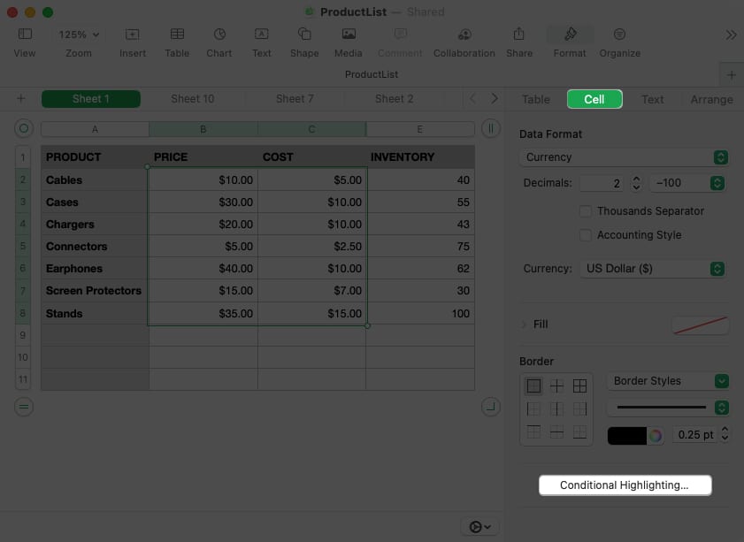
10. How one can apply conditional highlighting in Numbers
With conditional highlighting, you’ll be able to format your information routinely when it meets sure circumstances that you just arrange. As examples, you can also make numbers lower than one other quantity a sure font shade or dates after a selected date have a cell fill shade.
- Choose the cells you wish to apply the formatting to and click on Format to open the sidebar.
- Go to the Cell tab and decide Conditional Highlighting.
- On the high, click on Add a Rule. Select the rule sort on the left of the pop-up field.
You’ll be able to decide Quantity, Date, Textual content, Period, or Cell. - You’ll then see the out there circumstances for that cell sort to the appropriate. Choose an choice.
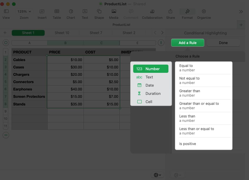
- Then, full the remaining particulars for the rule within the sidebar together with any further variables and the formatting you wish to apply.
- Click on Carried out once you end.

- To view, edit, or take away a conditional highlighting rule, reopen the Format sidebar and decide Present Highlighting Guidelines on the Cell tab.
Let’s have a look at an instance:
Right here, we’ll format numbers that equal 10 in pink font. Begin by selecting Quantity and Equal To.
Then, add the worth “10” and select Purple Textual content within the format drop-down checklist.
Now, every time a worth in our dataset is 10, we’ll see the pink font pop, making it straightforward to identify.
Do extra with Numbers on Mac
In case you’re a Mac person and wish to do extra with Apple Numbers, the following tips ought to enable you get began. And in case you have ideas of your individual you’d prefer to share or want to see us cowl one thing particular for Apple Numbers, tell us!
Learn extra:

Together with her BS in Data Expertise, Sandy labored for a few years within the IT trade as a Undertaking Supervisor, Division Supervisor, and PMO Lead. She wished to assist others learn the way expertise can enrich enterprise and private lives and has shared her strategies and how-tos throughout hundreds of articles.