
Python is a useful gizmo for becoming knowledge to the specified purposeful type and can be used to calculate the usual error for any argument in a perform match. In Python, to search out one of the best match of knowledge, and the optimum set of parameters for any user-defined perform, the “curve_fit()” methodology can be utilized that allows flexibility.
On this information, we’ll clarify:
What’s “SciPy” in Python?
The “SciPy” stands for “Scientific Python” which is the scientific computation open-source library and makes use of beneath the “NumPy”. It gives totally different utility features for sign processing, stats, and optimization, similar to “NumPy”.
What’s “Optimize Curve_fit” in Python?
To get the best-fit parameter, the “Optimize Curve_fit” perform can be utilized in Python. To acquire the optimized parameter for a supplied perform that matches the desired dataset, the “curve_fit()” perform can be utilized. It’s the freely obtainable library in SciPy that’s utilized to suit curves utilizing the nonlinear least squares.it takes the enter knowledge, output knowledge, and the specified perform title that’s to be employed.
Tips on how to Use Python’s “curve_fit” Operate to Match Information?
To suit any supplied knowledge set, first, import the required libraries, similar to “numpy”, “matplotlib.pyplot”, “curve_fit”, and “warnings”. Then, specified the state of warning as “ignore”
import numpy as np
import matplotlib.pyplot as plt
from scipy.optimize import curve_fit
import warnings
warnings.filterwarnings(‘ignore’)
Subsequent, we’ve got created the x-axis and y-axis values for a plot. Then, name an “np.asarray()” perform and move the beforehand created knowledge to generate an array. After that, name the “plt.plot()” perform with created arrays as parameters and the type of line through which we wish to show the plot:
yaxis = [ 11.7, 13.5, 14.5, 15.7, 16.1, 16.6, 16.0, 15.4, 14.4, 14.2, 12.7]
xaxis = np.asarray(xaxis)
yaxis = np.asarray(yaxis)
plt.plot(xaxis, yaxis, ‘o’)
Now, we outline the “Gaussian” perform equation in Python to search out the worth of “M” and “N” that finest match our knowledge. In response to the below-provided code, this perform will settle for as inputs the x-axis values and all of the arguments that will probably be finest match:
def Gauss(x, M, N):
y = M*np.exp(–1*N*x**2)
return y
Subsequent, name the “curve_fit()” perform that takes the perform that we have to match, the values of the x-axis and y-axis as arguments. Then, the optimized values of the “M” and “N” at the moment are saved within the listing parameters:
para, covariance = curve_fit(Gauss, xaxis, yaxis)
fit_M = para[0]
fit_N = para[1]
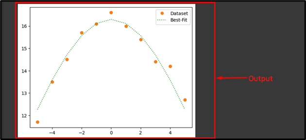
Now, we’ll calculate the values of the “y” through the use of our outlined perform and match values of “M” and “N”. After that, create a plot to match these calculated values to our specified knowledge with the “label” parameter with worth, perform variables, and plot line type. Lastly, name the “plt.present” perform to view the resultant plot:
fit_h = Gauss(xaxis, fit_M, fit_N)
plt.plot(xaxis, yaxis, ‘o’, label=‘Dataset’)
plt.plot(xaxis, fit_h, ‘:’, label=‘Greatest-Match’)
plt.legend()
plt.present()
Output

In response to the supplied output, we’ve got discovered one of the best match for our specified knowledge:
That’s all! We’ve briefly defined the “curve_fit()” perform in Python.
Conclusion
The “Optimize Curve_fit” perform is used to get the best-fit parameter in Python and to acquire the optimized parameter for a supplied perform that matches the desired dataset, the “curve_fit()” perform can be utilized. This information elaborated on the SciPy Optimize Curve_fit in Python.