Learn how to Use Matplotlib Pattern Line

The “Matplotlib” in style visualization library permits customers to create/make various varieties of graphs and charts. A vital characteristic of “Matplotlib” is the flexibility so as to add “Pattern Traces” to the graph, which helps visualize the development or relationship between variables in an efficient means.

On this article, we are going to discover the steps so as to add and customise a “Pattern Line” to a graph utilizing Matplotlib in Python by overlaying the next features:

Learn how to Add a Pattern Line to the Python Graph?

So as to add a development line to the graph utilizing “matplotlib”, the next steps are utilized in Python:

Step 1: Import the Required Libraries
Firstly, we have to import the required libraries, i.e., “matplotlib” and “numpy”. Here’s a code:

Step 2: Generate the Knowledge
Subsequent, we have to create/generate pattern information that we are able to make the most of to create/make a graph. We are able to create a “numpy” array containing the “X” and “Y” coordinates of the info factors. Right here is an instance code:

Step 3: Plot the Knowledge Factors
Now, we are able to plot the info factors using the “Matplotlib” library perform named “scatter()”. We are able to additionally customise the looks of the graph, such because the “coloration” and “measurement” of the info factors by way of the next code:

Step 4: Add a Pattern Line
So as to add a “Pattern Line” to the graph, calculate the “slope” and “intercept” of the road utilizing the numpy “polyfit()” perform. We are able to then use these values to create a line utilizing the Matplotlib “plot()” perform. The beneath code could be utilized to perform this:

Instance: Total Code
The ultimate step is to mix/joined all of the earlier steps and execute/run the total code:

Within the above code:

• The “plt.scatter()” perform is used to plot a scatter plot of “x” and “y” with purple dots and the scale of every dot as “50”.
• The “polyfit()” perform suits a line by means of the scatter plot information factors and returns the slope, and intercept of that line that are assigned to variables slope and intercept, respectively.
• The “plt.plot()” perform plots a straight line utilizing the slope and intercept values obtained from the “polyfit()” perform with blue coloration.

Output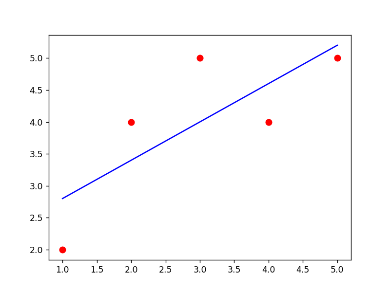

The above snippet verifies that the development line has been added to the enter graph.

Learn how to Customise the Pattern Line in Python?

To customise the looks of the development line, such because the “line width” and “fashion”, a number of arguments of “matplotlib” capabilities are utilized in Python. We are able to do that by passing extra arguments to the “plot()” perform. Let’s customise the development line utilizing the next examples:

Instance 1: Including “Line Width” and “Type”
The beneath code is used so as to add “linewidth” and “fashion” to the required “Pattern Line”:

Within the above code block, the “plt.plot()” perform takes the “linewidth=2”, and “linestyle= ‘dashed’” attributes as its parameters, and customizes the created development line.

Output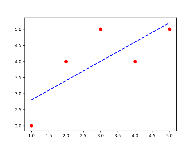

The custom-made development line has been created within the above output appropriately.

Instance 2: Including “Labels” and “Title”
The required labels to the “X” and “Y” axis, and a “title” will also be added to the graph utilizing the matplotlib “xlabel”, “ylabel”, and “title()” capabilities. The beneath instance code could be utilized to perform this:

Within the above code, the “plt.xlabel()”, “plt.ylabel()” and “plt.title()” capabilities are used to label the x-axes and y-axes, and add a title, respectively.

Output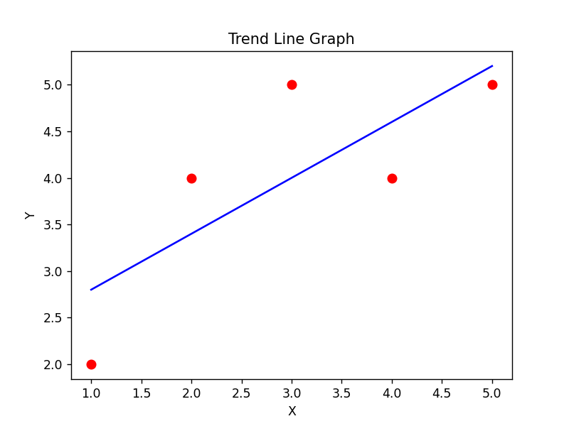

The above output exhibits that the trendline plot graph has been custom-made with the “x” and “y” labeling, and a title.

Instance 3: Use Matplotlib to Create a Polynomial Trendline
In Python, a “Polynomial Trendline” is a line of finest match that represents a polynomial equation of diploma “n” (the place n is any constructive integer) that minimizes the gap between the info factors and the road.

The “polyfit()” perform is used to calculate the coefficients of the polynomial equation and the “poly1d()” perform is used to create a polynomial object that can be utilized to plot the trendline on a graph. The next code is utilized to create/make a polynomial trendline:

Within the above traces of code:

• The “plt.scatter()” perform is used to plot a scatter plot of given “x” and “y” values with purple coloration and a measurement of “50”.
• The “numpy.polyfit()” perform suits a second-degree polynomial curve to the info.
• The “numpy.poly1d()” perform creates a polynomial perform and assigns it to a variable “p”.
• Lastly, the “plt.plot()” perform plots the polynomial curve on prime of the scatter plot.

Output

This snippet implies that the polynomial trendline has been added to the graph efficiently.

Conclusion

In Python, the “Matplotlib” library capabilities “plt.polyfit()” and “plt.plot()” are used collectively so as to add a linear “Pattern Line” to a graph and these capabilities could be utilized with the “poly1d()” perform to create a polynomial “Tread Line”. To customise the development line, varied arguments similar to “linewidth”, “linestyle”, and “coloration”, and so forth. are handed to the “plt.plot()” perform. This Python tutorial supplies an in-depth information on including a development line to a graph utilizing acceptable examples.