
The shifting common, also referred to as a rolling or working common, is a time-series information evaluation instrument that computes the averages of distinct subsets of your complete dataset. It’s also referred to as a shifting imply (MM) or rolling imply as a result of it consists of calculating the imply of the dataset over a sure interval. The shifting common may be computed in quite a lot of strategies, considered one of which is to pick an outlined subset from a complete sequence of numbers.
Pandas DataFrame.Ewm()
EWMA gives extra weight to present observations or much less weight to information because it strikes additional again in time, permitting it to file the latest developments comparatively faster than the opposite methods of discovering averages. The “DataFrame.ewm()” Pandas methodology is used to carry out EMA.
Syntax:
pandas.DataFrame.ewm(com=None,span=None,halflife=None,alpha=None,min_periods=0,
alter=True,ignore_na=False,axis=0).imply()
Parameters:
-
- The primary parameter, “com”, is the discount within the heart of weight.
- The “span” is the span-related degradation.
- The “halflife” represents the halflife’s decline.
- The “alpha” parameter is a smoothing component whose worth ranges from 0 to 1 inclusively. The “min_periods” specifies the minimal variety of observations in a timeframe that’s wanted to supply a worth. In any other case, NA is returned.
- To right for an imbalance in relative weightings like “alter”, divide by a declining adjustment issue into the beginning intervals.
- When calculating weights, the “ignore_na” disregard the lacking values.
- The “axis” is the suitable axis to make use of. The rows are recognized by the quantity 0, whereas the columns are recognized by the worth 1.
Instance 1: With Span Parameter
On this instance, we’ve got an analytics DataFrame that retailer the Firm Product inventory data. We have now Product, amount and value columns, and firm must estimate the exponential shifting common with a span of 5 days.
# Create pandas dataframe for calculating Exponential Shifting Common
# with 3 columns.
analytics=pandas.DataFrame({‘Product’:[11,22,33,44,55,66,77,88,99,110],
‘amount’:[200,455,800,900,900,122,400,700,80,500],
‘value’:[2400,4500,5090,600,8000,7800,1100,2233,500,1100]})
print(analytics)
print()
# Calculate Exponential Shifting Common for five days
analytics[‘5 Day EWM’]=analytics[‘quantity’].ewm(span=5).imply()
print(analytics)
Output:
0 11 200 2400
1 22 455 4500
2 33 800 5090
3 44 900 600
4 55 900 8000
5 66 122 7800
6 77 400 1100
7 88 700 2233
8 99 80 500
9 110 500 1100
Product amount value 5 Day EWM
0 11 200 2400 200.000000
1 22 455 4500 353.000000
2 33 800 5090 564.736842
3 44 900 600 704.000000
4 55 900 8000 779.241706
5 66 122 7800 539.076692
6 77 400 1100 489.835843
7 88 700 2233 562.734972
8 99 80 500 397.525846
9 110 500 1100 432.286704
Rationalization:
Within the first output, we displayed your complete analytics. Within the second output, we calculate the exponential shifting common for the amount column and retailer the values within the “5 day EWM” column.
Instance 2: Visualize the EWM
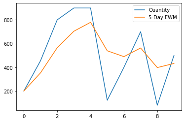
Let’s visualize the exponential shifting common for the “amount” column over a span of 5 days utilizing the Matplotlib module.
import pandas
analytics=pandas.DataFrame({‘Product’:[11,22,33,44,55,66,77,88,99,110],
‘amount’:[200,455,800,900,900,122,400,700,80,500],
‘value’:[2400,4500,5090,600,8000,7800,1100,2233,500,1100]})
# Plot the precise amount
pyplot.plot(analytics[‘quantity’],label=‘Amount’)
# Calculate Exponential Shifting Common for five days
analytics[‘5 Day EWM’]=analytics[‘quantity’].ewm(span=5).imply()
# Plot the 5 Day exponential shifting common amount
pyplot.plot(analytics[‘5 Day EWM’],label=‘5-Day EWM’)
# Set the legend to 1
pyplot.legend(loc=1)
Output:
<matplotlib.legend.Legend at 0x7f39f0f220a0>
Rationalization:
We calculate the exponential shifting common for the amount column and retailer the values in “5 day EWM” column. Now, you’ll be able to see that within the graph, the blue line signifies the precise “amount” and the orange shade signifies the Exponential Shifting Common with a span of 5 days.
Instance 3: With Span and Modify Parameters
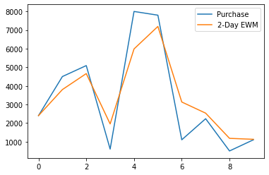
Estimate the exponential shifting common for the “value” column with a span of two days by setting the alter to False and visualize it.
import pandas
analytics=pandas.DataFrame({‘Product’:[11,22,33,44,55,66,77,88,99,110],
‘amount’:[200,455,800,900,900,122,400,700,80,500],
‘value’:[2400,4500,5090,600,8000,7800,1100,2233,500,1100]})
# Plot the precise value
pyplot.plot(analytics[‘cost’],label=‘Buy’)
# Calculate Exponential Shifting Common for two days
analytics[‘2 Day EWM’]=analytics[‘cost’].ewm(span=2,alter=False).imply()
# Plot the two Day exponential shifting common value
pyplot.plot(analytics[‘2 Day EWM’],label=‘2-Day EWM’)
# Set the legend to 1
pyplot.legend(loc=1)
print(analytics)
Output:
Product amount value 2 Day EWM
0 11 200 2400 2400.000000
1 22 455 4500 3800.000000
2 33 800 5090 4660.000000
3 44 900 600 1953.333333
4 55 900 8000 5984.444444
5 66 122 7800 7194.814815
6 77 400 1100 3131.604938
7 88 700 2233 2532.534979
8 99 80 500 1177.511660
9 110 500 1100 1125.837220
Rationalization:
We retailer the values within the “2 day EWM” column for value and show. Lastly, we visualize utilizing the Matplotlib Pyplot.
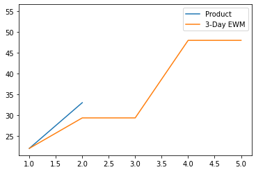
Instance 4: With Ignore_Na Parameter
See the exponential shifting common for the “Product” column having None values with a span of three days by setting the ignore_na to False.
import pandas
analytics=pandas.DataFrame({‘Product’:[None,22,33,None,55,None],
‘amount’:[200,455,None,900,900,122]})
# Plot the precise value
pyplot.plot(analytics[‘Product’],label=‘Product’)
# Calculate Exponential Shifting Common with span of three days with out ignoring NaN values.
analytics[‘3 Day EWM with NaN’]=analytics[‘Product’].ewm(span=3,ignore_na=False).imply()
# Plot the three Day exponential shifting common Product
pyplot.plot(analytics[‘3 Day EWM with NaN’],label=‘3-Day EWM’)
# Set the legend to 1
pyplot.legend(loc=1)
Output:
<matplotlib.legend.Legend at 0x7f841a59a190>
Conclusion
The idea of calculating the exponential weighted shifting common is mentioned on this article. Within the introduction part of this writing, we defined the concept of EWM. The “DataFrame.ewm().imply()” Pandas methodology is supplied with all its parameters that are briefly described. We carried out 4 examples. The fundamental methods for computing EWM are elaborated on on this studying.