
“Rolling correlations are obtained by calculating the correlations amongst two time collection utilizing a rolling window. We are able to determine if two correlated time collection diverge from each other over time utilizing rolling correlations.”
Discovering the rolling correlation on a Pandas DataFrame will be performed utilizing the “DataFrame_object.rolling().corr()” methodology. On this illustration, we’ll study to compute the rolling correlation on a Pandas DataFrame with the essential method.
Syntax:
On two DataFrames:
DataFrame_object1.rolling(width).corr(DataFrame_object2)
(OR)
On two columns in a DataFrame:
DataFrame_object[‘column1’].rolling(width).corr(DataFrame_object[‘column2’])
The vital factor to recollect whereas specifying the values for the columns is that the size of the values for all of the columns that are contained within the DataFrame should have to be equal. If we put an unequal size of values, this system won’t execute.
Instance 1: Correlate Column1 vs Column2
Let’s create a DataFrame with 3 columns and 10 rows and correlate the amount with the fee column for two days.
# Create pandas dataframe for calculating Correlation
# with 3 columns.
analytics=pandas.DataFrame({‘Product’:[11,22,33,44,55,66,77,88,99,110],
‘amount’:[200,455,800,900,900,122,400,700,80,500],
‘value’:[2400,4500,5090,600,8000,7800,1100,2233,500,1100]})
# Correlate amount with value column for two days.
analytics[‘Correlated’]=analytics[‘quantity’].rolling(2).corr(analytics[‘cost’])
print(analytics)
Output:
Product amount value Correlated
0 11 200 2400 NaN
1 22 455 4500 1.0
2 33 800 5090 1.0
3 44 900 600 –1.0
4 55 900 8000 NaN
5 66 122 7800 1.0
6 77 400 1100 –1.0
7 88 700 2233 1.0
8 99 80 500 1.0
9 110 500 1100 1.0
The correlation for two days, 200 to 400, is NaN and so forth that are positioned within the “Correlated” column.
Instance 2: Visualization
Let’s create a DataFrame with 3 columns and 5 rows and correlate the “Gross sales” vs “Product_likes”.
Use the Seaborn to view the correlation in a graph and get the Pearson correlation coefficient.
import seaborn
from scipy import stats
# Create pandas dataframe for calculating Correlation
# with 3 columns.
analytics=pandas.DataFrame({‘Product identify’:[‘tv’,‘steel’,‘plastic’,‘leather’,‘others’],
‘Product_likes’:[100,20,45,67,9],
‘Gross sales’:[2300,890,1400,1800,200]})
print(analytics)
print()
# See the coefficient of correlation
print(stats.pearsonr(analytics[‘Sales’], analytics[‘Product_likes’]))
print()
# Now see the Correlation Gross sales vs Product_likes
seaborn.lmplot(x=“Gross sales”, y=“Product_likes”, knowledge=analytics)
Output:
0 television 100 2300
1 metal 20 890
2 plastic 45 1400
3 leather-based 67 1800
4 others 9 200
(0.9704208315867275, 0.006079620327457793)
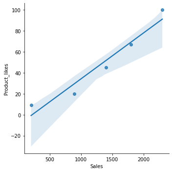
Now, you may see the correlation between Gross sales and Product_likes.
Let’s now get the rolling correlation for these two columns for 3 days.
Code for Instance 2:
# Correlate Gross sales with Product_likes column for five days.
analytics[‘Correlated’]=analytics[‘Sales’].rolling(3).corr(analytics[‘Product_likes’])
print(analytics)
Output:
Product identify Product_likes Gross sales Correlated
0 television 100 2300 NaN
1 metal 20 890 NaN
2 plastic 45 1400 0.998496
3 leather-based 67 1800 0.999461
4 others 9 200 0.989855
You may see that these two columns are extremely correlated.
Instance 3: Totally different DataFrames
Let’s create 2 DataFrames with 1 column every and correlate them.
import seaborn
from scipy import stats
analytics1=pandas.DataFrame({ ‘Gross sales’:[2300,890,1400,1800,200,2000,340,56,78,0]})
analytics2=pandas.DataFrame({‘Product_likes’:[100,20,45,67,9,90,8,1,3,0]})
# See the coefficient of correlation for the above two DataFrames
print(stats.pearsonr(analytics1[‘Sales’], analytics2[‘Product_likes’]))
# Correlate Gross sales with Product_likes DataFrame
print(analytics1[‘Sales’].rolling(5).corr(analytics2[‘Product_likes’]))
Output:
(0.9806646612423284, 5.97410226154508e-07)
0 NaN
1 NaN
2 NaN
3 NaN
4 0.970421
5 0.956484
6 0.976242
7 0.990068
8 0.996854
9 0.996954
dtype: float64
You may see that these two columns are extremely correlated.
Conclusion
This dialogue revolves round calculating the rolling window after which discovering the correlation of a Pandas DataFrame. To place each these ideas into apply, Pandas gives a sensible “DataFrame.rolling().corr()” methodology. For the learner’s comfort to grasp the method higher, we’ve got given three virtually carried out examples together with visualization and Searborn module. Every instance is drawn-out with an in depth rationalization of the steps. You may both apply it to totally different columns in a single DataFrame or you could use the identical columns from totally different DataFrames; all of it depends upon your necessities.